Headed to AACR? Schedule time to connect with us at bd@ozette.com
Evan Greene, Chief Officer Applied Sciences
Generating single-stain controls is a critical step for the correct unmixing of spectral cytometry datasets. This is because unmixing relies on the fundamental assumption that the measured performance of fluorochromes in control samples accurately represents the performance of those same dyes when they stain experimental samples as part of a complete panel.
One common way this assumption is violated is cross-contamination of control samples. Whether it is caused by pipetting error or carryover during acquisition, if not corrected, contamination can compromise outputs for all samples that use the afflicted control(s) for unmixing.
How do you know if a control is contaminated? Opportunities for detection are provided by the visualizations produced in a given workflow. In this post, we will compare the Resolve workflow to a conventional workflow, and demonstrate tooling built into Resolve that helps identify and remediate contamination in controls so that they may still be used for the correct unmixing of full stained samples.
Before we built Resolve, our lab would follow a conventional workflow and use the instrument-provided unmixing tool. In this workflow, we’d typically set a lineage gate followed by a positive gate on each control file, and then examine the provided ribbon plots and estimated spectra for evidence of problems.
A typical control would produce a visualization like the following, where we see data from a control stained by BUV737 conjugated to anti-CD127.
Here, the range of intensities on detectors UV7, V6, YG1 (and their neighbors) indicate a serious problem has occurred. When observed, experienced operators may recognize one likely cause is contamination, and attempt to remediate it via gating. Gating as remediation is only possible when the contaminating dye is dissimilar: one needs to select a detector where the contaminant emits light and the intended fluor does not in order to set a remediation gate.
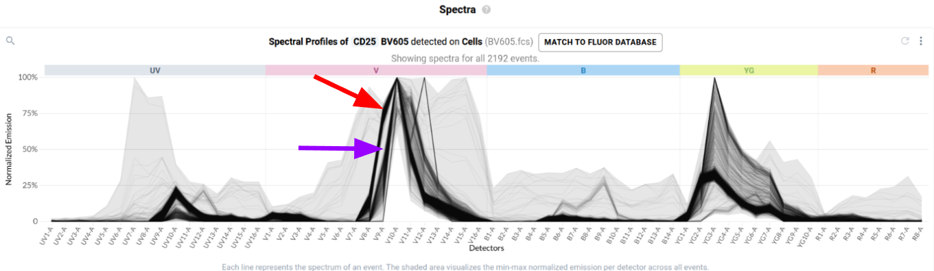
As panels expand, however, the fluorophores used in a panel increasingly crowd the emissions range, and the chance of similar dyes contaminating one another increases. Consider the following plot generated by a control for BV605 conjugated to anti-CD25.
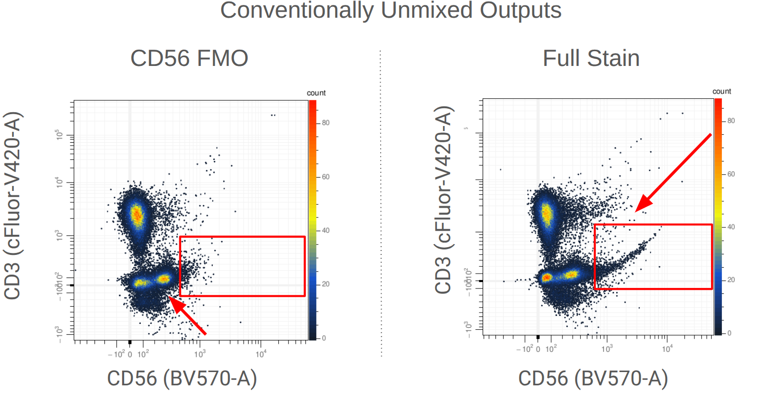
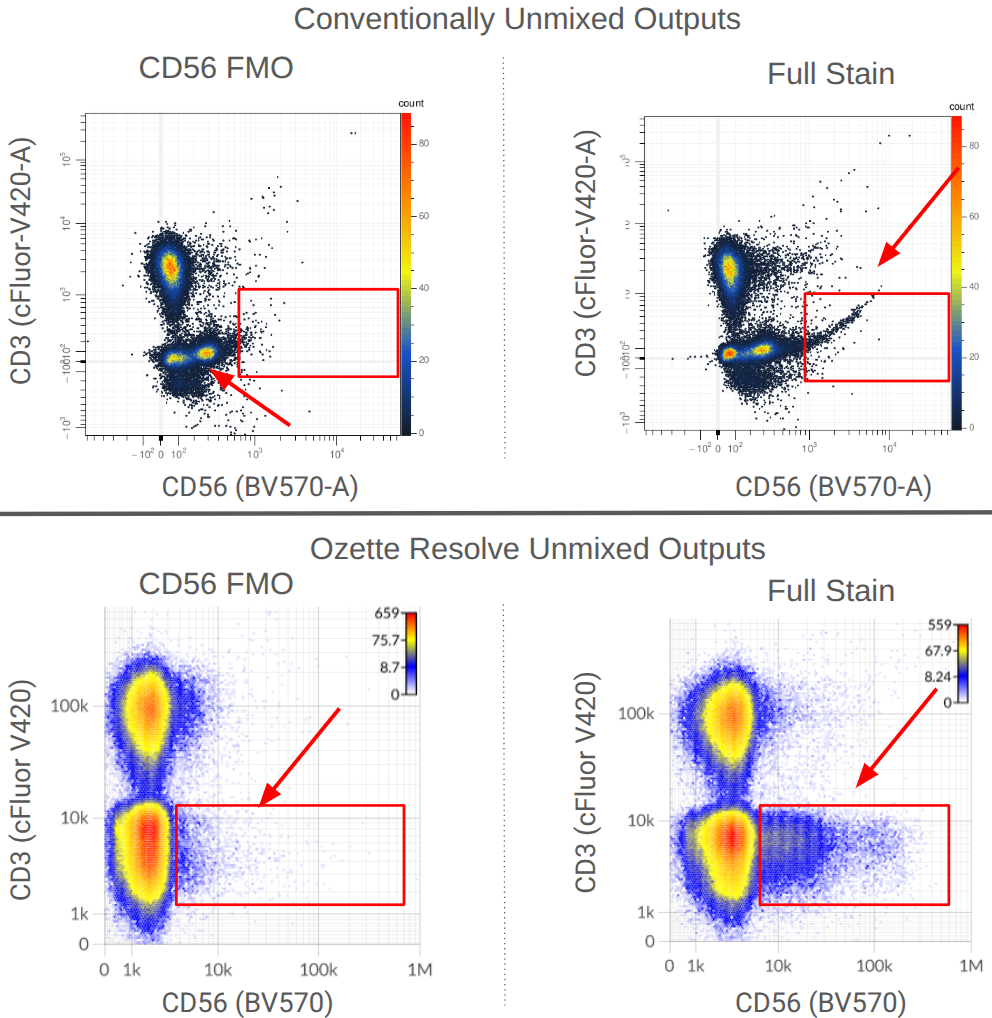
Is this control capturing the performance of the fluorophore when stained at the panel’s titre? Or do problems lurk beneath the surface? If one doesn’t know there are problems to fix, and one doesn’t know how to implement a fix when problems are detected, they are left in the position of having to unmix full stained data with the controls at hand. In these data, we can infer problems are present by looking at N x 1 plots of the conventionally unmixed outputs, where we can see odd patterns like the following emerge.
When an analyst encounters these kinds of patterns in their unmixed outputs, they are put in a difficult position: are the double peaks and the upward-tilting expression tail in the full-stain sample biological signals or artifacts of the unmixing process? By generating FMOs, we can interpret the double peak as an unmixing artifact (though this would not be possible if you are unable to routinely generate FMOs). But if the upward tail seen in the full stain plot is an unmixing artifact, it can cause problems in downstream analysis: if you aim to characterize NKT cells, for example, this kind of pattern can inflate false-positive or false-negative rates.
Because of this risk, analysts often attempt to address such artifacts through manual compensation: they apply a ‘correction matrix’ to the unmixed files. This is not recommended for many reasons. Among them, compensation introduces subjective bias into the analysis, and can introduce errors into other parameters. The ideal way to address this kind of artifact is in the unmixing step itself, but this also places analysts in a difficult spot: which controls caused the problems, and can the controls be salvaged?
The Resolve “control set” workflow is designed to make identification and remediation of contaminated control files easy. A “control set” is simply a collection of single stained and unstained control files that can be used to unmix fully stained experimental samples. The workflow is flexible (and its flexibility will be explored in follow-on posts), but in its simplest incarnation a control set is defined by a single unstained control and one control per fluorophore in a panel. We will use this type of control set to illustrate the workflow in this post.
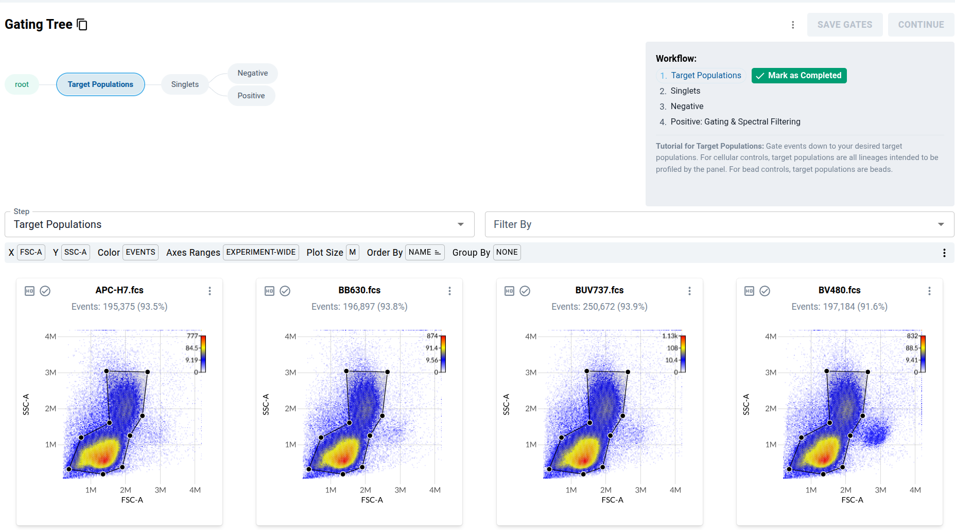
The workflow begins with a template gating tree being applied to each control. This gating tree allows users to identify events within each control file that are profiled by the panel (the system can be used for open-ended gating if needed).
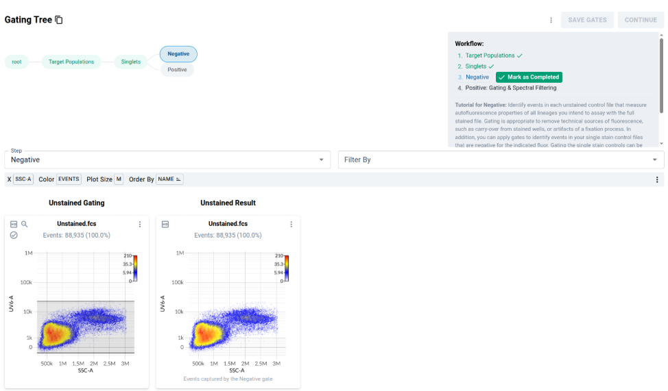
Once you have gated down to events within the targeted lineages, users are then provided a view of their unstained controls. They may apply gates in this step to remove contaminants from their unstained files, or to gate “internal negatives” within their single stained controls. This latter capability is particularly useful when a user has exclusively generated synthetic mixed bead controls.
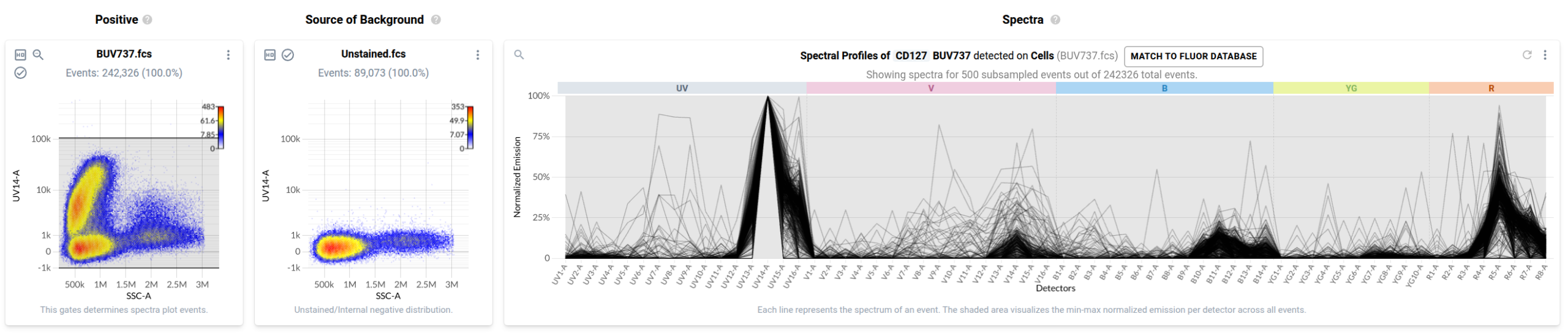
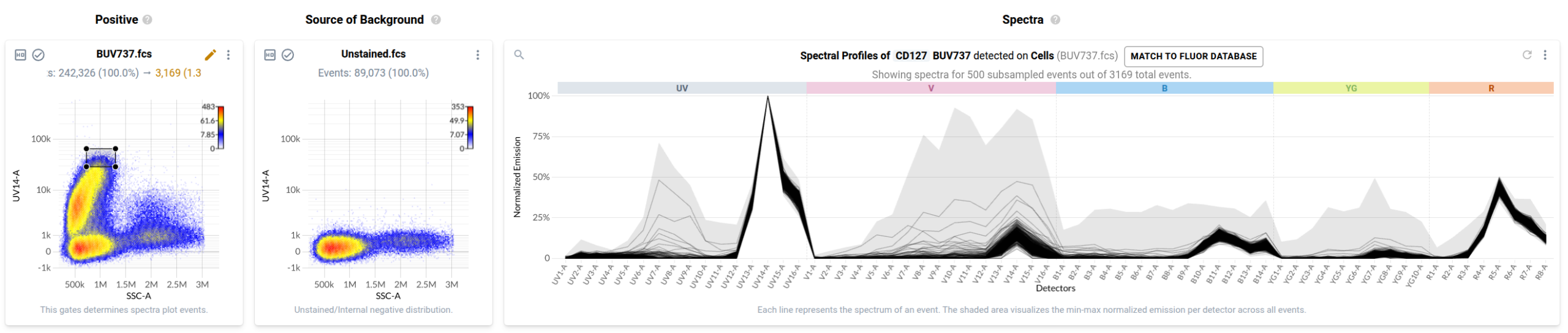
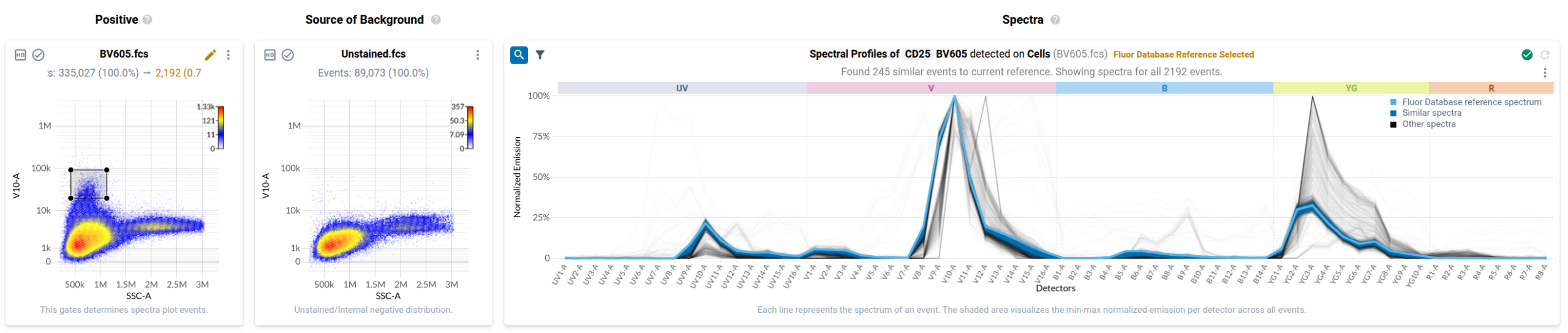
In the first component labelled “Positive”, the plot shows the gated lymphocytes and monocytes in this control file, with side scatter on the x-axis, and the peak detector on the y-axis. In the second component labeled “Source of Background”, the plot shows data from the unstained control on the same parameters, to help users interpret which events are above the unstained background.
The third component labelled “Spectra” is the spectral plot, which shows the estimated spectra for the events within the positive gate. By default it shows a random sample of 500 events among the ~242k measured in the file (the plot can be updated to show more or all events). The gray background color saturates the plot, which indicates that there are events in this dataset with fluorescence emission that peak across the entire detector array. Since by default we include negative events, this makes sense: those events are unlabelled, and their spectra (produced by autofluorescence) can fluctuate randomly across the device.
We can update the gate on the positives to only capture bright (presumably stained) events, and we see that the spectral plot updates to reflect this data.
Now we can see that among events that have likely been labelled, the gray background showing the span of spectra is more centrally concentrated among the expected emission region (the white background indicates no events have spectra with normalized emission at that level within the gate). On some detectors, however, there are still visible outliers among these events. Resolve provides several tools to help further purify the signals measured in the control.
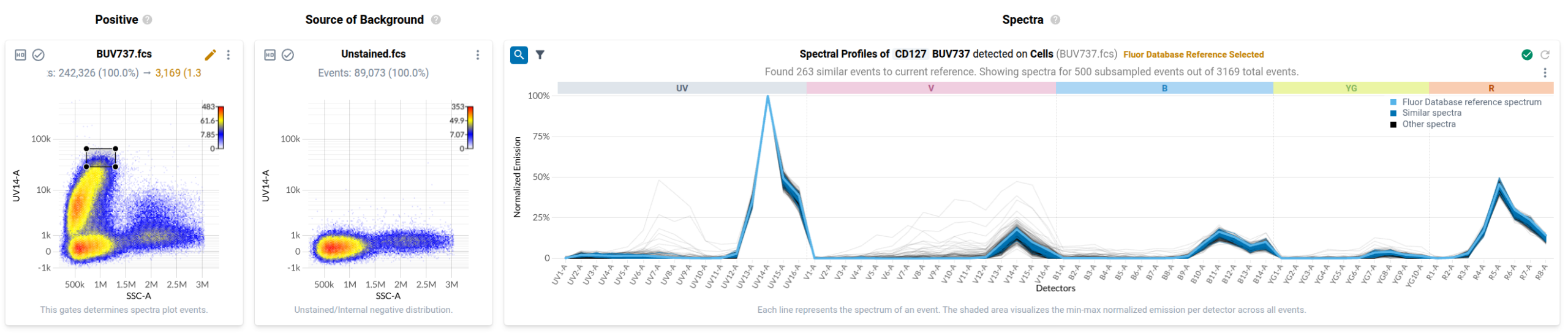
One powerful tool is the ability to compare the gated events in the control to a reference spectrum. The reference spectra in Resolve were generated by the Ozette lab team in Seattle. Our lab team has generated references for a large number of fluorophores, and you can have Resolve find the events in your file that are most similar to this reference by clicking the button at the top of the spectral plot.
After clicking this button, the plot updates to show the shape of the reference spectrum on the plot, and further shows a filtration of events within the gate: it now shows the subset of events in the sample that are close to the reference spectrum in blue, and excluded events in gray tones.
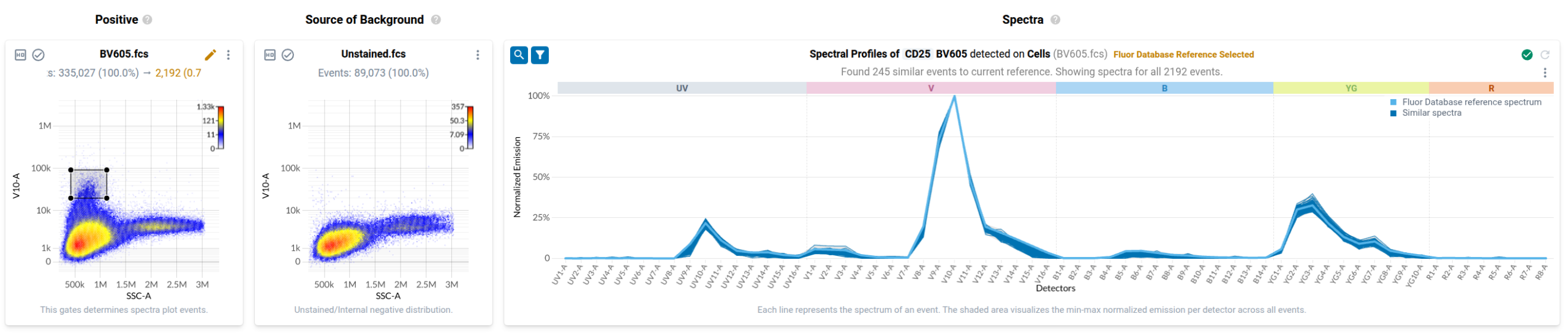
The filtered plot now shows several hundred events within the gate that have similar shapes to the reference spectrum. It’s important to note that the reference spectrum is only a starting point: experimental conditions can produce changes in the shape and relative height of secondary (and tertiary, etc.) emission peaks in controls. In such cases, the reference spectrum is still helpful to help start the workflow, but users are encouraged to manually select a positive empirical reference in their data and then filter against that selection in such cases. This is because the empirical evidence in the control offers the best information about the emission profile of each fluorophore on their device in their experimental conditions.
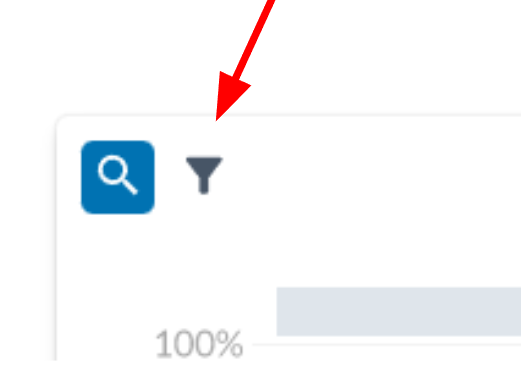
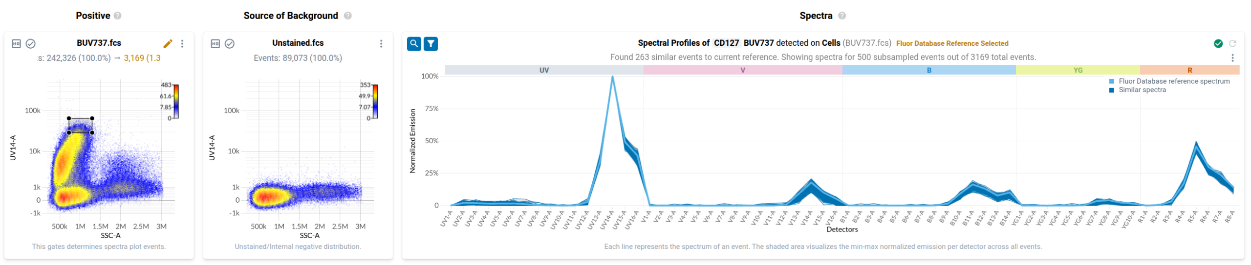
After the spectral filtering is carried out, outliers in gray are still visible on the spectral plot. These can be removed from the view by clicking the funnel icon in the upper-left corner of the plot.
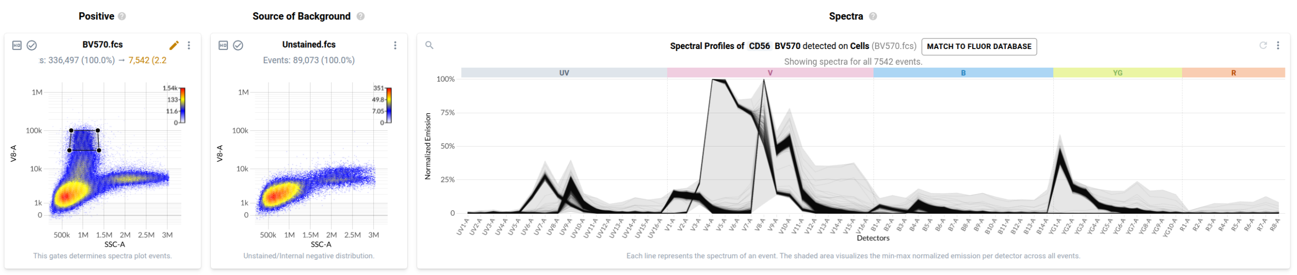
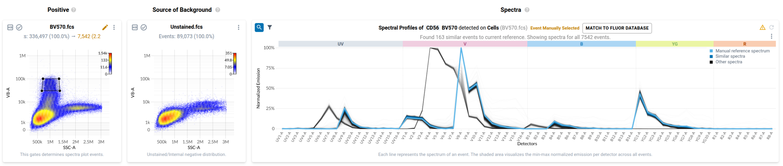
Now that we’ve seen the workflow carried out for an uncontaminated file, let’s examine how Resolve helps identify and remediate contamination within a single stain control. We return to the control labelled with anti-CD56 conjugated to BV570, where earlier we noted it has been contaminated by events labelled with anti-CD45RA conjugated to BV480. After gating positives in this workflow we can see the clear mixture of the BV570 and BV480 emission patterns among events in the positive gate.
By selecting and filtering relative to a BV570 positive event, we can easily exclude the contaminating BV480 signal.
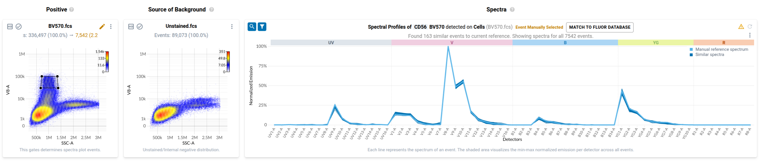
We can confirm BV480 is excluded by updating the plot to show only the positive events.
The events in this last view are the BV570 positive events that will be used to unmix full stained data.
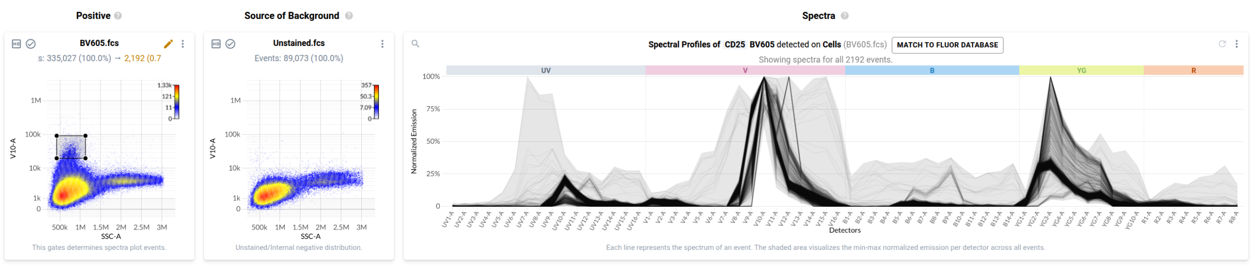
As a final example, we return to the control labelled with anti-CD25 conjugated to BV605. The spectral plot in Resolve makes it clear that there are two similar but distinct spectral patterns in the control file.
This control has in fact been contaminated by events labelled with anti-CD4 conjugated to cFluor V610. These are similar fluorophores, but in Resolve you can see distinct patterns of emission across the violet detectors contaminating the file.
The three examples discussed above show how the Resolve spectral filtering workflow identifies true positive events in both contaminated and uncontaminated files. It is the same workflow in all cases, and it makes it easy to find and fix contamination errors by filtering the contaminants out. The cumulative effect of filtering down to true positive events becomes clear when we unmix fully stained data and re-examine the earlier pair plot showing all events in each file.
Where before we saw an artifactual double peak and expression tail curving upwards, in the Resolve outputs these unmixing artifacts are eliminated. We know these are artifacts because we see them in the conventionally unmixed FMO control. Resolve spectral filtering is one reason these errors are absent. Another reason is the mathematical model Resolve uses to carry out unmixing itself, which we will explore in the next post on this blog. Here, it suffices to note that the Resolve model will only produce non-negative outputs, and that the scale of the output differs by design: the model is specified so the unmixed output for an event recovers the total raw measured signal across all detectors (on average) for that event. Because of this, the scale of Resolve output typically differs across parameters from conventional approaches (which you can see in the above plot).
In this post we have seen how the Resolve spectral filtering workflow can automatically surface and fix cross-contamination errors that occur in cytometry experiments. As this kind of error is inevitable (despite best efforts, every team will make occasional mistakes at the bench if they perform experiments regularly), it’s a particularly powerful component of Resolve since it prevents these mistakes from introducing error into the unmixed outputs. This also can save costs at the bench: users can use contaminated controls they’ve already generated for optimal unmixing by filtering out contaminants in Resolve, so they don’t have to go back to the lab to generate another set of reference controls.
In our next post, we will discuss how the mathematical model used by Ozette Resolve takes advantage of the spectral filtering workflow to generate high-quality outputs. In the meantime, if you’d like to try the spectral filtering workflow with Resolve today, try our 30-day free demo at https://ozette.com/biological-insights/.